Excel Tips and Tricks: 2012

How to split a cell diagonally

Let say we need to split the cells diagonally. Mainly when we want make a nice looking table.

Let say we need a table showing machine numbers and outputs per day.

As you can see event though the data can be represented properly, the presentation part is not very good as there will be empty cells (colored in yellow).

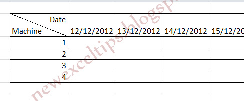
A nicer table should have "Date" and "Machine" in the same cell. Just like the one below,

Let see how to do this.

1. Right click on the cell where we want to put "Date" and "Machine" and click on Format cells.

Select "Border" and click on the diagonal border.

Click "OK"

Set the cell's Horizontal Alignment to "left" and vertical alignment to "center".

Type in "Date" then Hit "Alt+Enter". The type in "Machine".

Use the space bar to push the "Date" to right to get what we want.

If you want to have two colors for the split area you can try the "Fill effects". Choose "two colors" and "Diagonal Down". This is the best I can think of.

Please note if you want to use the value (date machine), this is not the method.

As always love to have your comments.

How to use #N/A to create line plots look more presentable

Let's look at the example below. The table showing rejects (column B), output (column C) and reject percentage (column D). Reject percentage = B2/C2.

Day	Rejects	Output	Reject Parentage
1	5	300	1.67%
2	80	400	20.00%
3	30	350	8.57%
4	0	0	#DIV/0!
5	45	455	9.89%
6	67	340	19.71%
7	43	360	11.94%
8	89	400	22.25%
9	23	320	7.19%
10	56	330	16.97%

Note on the fourth day there was no production. So we get an error in the reject percentage column. If we plot the reject percentage, We will get,

On day four there is no production and so no rejects.
The plot is not accurate as it shows reject percentage as zero.

Ideally the plot should ignore day 4. To achieve this we need to change the formula in column D.

=IF(ISERROR(B2/C2)=TRUE,#N/A,B2/C2)

Now the table looks like,

Day	Rejects	Output	Reject Parentage
1	5	300	1.67%
2	80	400	20.00%
3	30	350	8.57%
4	0	0	#N/A
5	45	455	9.89%
6	67	340	19.71%
7	43	360	11.94%
8	89	400	22.25%
9	23	320	7.19%
10	56	330	16.97%

Now plot the reject percentage again.

Now the plot ignores day 4 and it shows no data point on day 4.

As always love to have your comments.

How to find the position of last of the multiple characters in a cell

Let's look at the example here. There are cells that contain something similar to

drive1\folder1\file1023
drive2\folder2\subfolder2\file256
drive10\file34
..
..
..

The text after the last "/" is to be extracted, the result should be,

file1023
file256
file34
..
..

To do that you need position of the last "/". FIND function alone is not use because of two unknowns, one how many "/" s are there and second what is the "start number" to use.

But it is possible using RIGHT, FIND, SUBSTITUTE and LEN.
Let's say drive1\folder1\file1023 is in cell A1.

The formula to get file1023 will be

RIGHT(A1,LEN(A1)-FIND("#",SUBSTITUTE(A1,"/","#",LEN(A1)-LEN(SUBSTITUTE(A1,"/","")))))

Note '#' can be any character.

Let's analyse the formula to see how it works. The formula works using [instance_num] (Which is not available in FIND function) of the SUBSTITUTE function and substituting "\" with "" (or nothing).

SUBSTITUTE(text, old_text, new_text, [instance_num])

Lets look at the formula from right to left.

LEN(SUBSTITUTE(A1,"\","")) will give number of characters after replacing "\" with "".

LEN(A1) will give number of characters before any change.

The difference is the number of "\" in the cell, in this example 2.

SUBSTITUTE(A1,"\","#",LEN(A1)-LEN(SUBSTITUTE(A1,"\",""))) will replace only the last "\" with "#" using 2 as the [instance_num ]. Now "#" is in the last "\" position.

Now using FIND the position of "#" can be found, in this example 15.

Using RIGHT formula with identified position of the "#" it is possible to extract file 1023.

LEN(SUBSTITUTE(A1,"\",""))	21
LEN(A1)	23
LEN(A1)-LEN(SUBSTITUTE(A1,"\",""))	2
SUBSTITUTE(A1,"\","#",LEN(A1)-LEN(SUBSTITUTE(A1,"\","")))	drive1\folder1#file1023
FIND("#",SUBSTITUTE(A1,"\","#",LEN(A1)-LEN(SUBSTITUTE(A1,"\",""))))	15

RIGHT(A1,LEN(A1)-FIND("#",SUBSTITUTE(A1,"/","#",LEN(A1)-LEN(SUBSTITUTE(A1,"/","")))))	file1023

Please let me know if you have any concerns or questions.

How to find duplicates in column without deleting them

It is a common requirement to find duplicates, in most cases the duplicates need to be deleted, but in some cases the duplicates need to be kept.

Excel 2010 (even 2007?) got the feature under "DATA" to remove duplicate entries in column(s), called Remove Duplicates.

The issue with this tool it removes the duplicates and do not give more details.

If you want to mark the duplicates or want to VLOOKUP unique values you need use COUNTIF.

Let's see the example below,

There are many duplicate entries i column D. If you want to put "Duplicate" in column C, use

=IF(COUNTIF($D$2:$D$45,D2)>1,"DUPLICATE","")

The result will be,

Important to note, if there is two or more values, all considered "DUPLICATE". This will not help if you are looking to use unique values. For example if you try to index the unique values, let's say in column B.

You may want to use,

=IF(C2="DUPLICATE","",MAX(B$1:B1)+1)

The result will be a "1" in B15. In other words there is only one unique value in column D. But we know it is not true. To solve this we need to change the COUNTIF slightly.

Instead of

=IF(COUNTIF($D$2:$D$45,D2)>1,"DUPLICATE","")

We will use,

=IF(COUNTIF(D$2:D2,D2)>1,"DUPLICATE","")

and the result is,

Now you can use VLOOKUP to pull the unique values, Vlookup(1,B:D,2,FALSE) and so on.

The Key Point is to leave the first instance of the duplicates as "Unique".

There will be lot of other ways to do the same.
I will be happy to have any feedback.

How to use COLUMN and COLUMNS functions.

Lets look at the two functions which sound similar but give different results. COLUMN gives the position of the column and COLUMNS counts the number of columns in a range.

Let's see the syntax.

COLUMN([reference])

COLUMNS(array)

Examples
COLUMN(F2) = 6
COLUMN() = will give the column position of the cell where the function is.

COLUMNS(F10:I14) = 4

One use of the COLUMN function is with VLOOKUP.
Consider the example below, A table of outputs of different machines in different days.

Now I want to pull only machine 3 data to another place using VLOOKUP. First I key in Machine 3 in A6 for this example.
I need the values in column I to L to appear in column B to E.

I can key in =VLOOKUP($A6,$H:$L,2,FALSE) in B6, =VLOOKUP($A6,$H:$L,3,FALSE) in C5 and so on.
But I need to keep changing the col_index_num for every column. If you are working with a large table it can be tedious work.

Here we can use column function to make it automatic when we drag the function. The formula looks like this,

in B6 =VLOOKUP($A6,$H:$L,COLUMN(I:I)-7,FALSE)

COLUMN(I:I)-7 = 2

When you drag the function,
in C6 =VLOOKUP($A6,$H:$L,COLUMN(J:J)-7,FALSE)
in D6 =VLOOKUP($A6,$H:$L,COLUMN(K:K)-7,FALSE)
in E6 =VLOOKUP($A6,$H:$L,COLUMN(L:L)-7,FALSE)

You can use COLUMNS(A:G) instead of 7
=VLOOKUP($A6,$H:$L,COLUMN(I:I)-COLUMNS(A:G),FALSE)

Depending on the table location and where you want to pull the data the function for col_index_num will change.

Please let me know comments/feedback.

Excel Tips - How to use CHOOSE function

Another simple function which seems nothing much of a use at the first look. But it can be used choose from a predetermined list.

Syntax

CHOOSE(index_num, value1, [value2], ...)

index_num and value1 and necessary. value2 to value255 (excel 2010) is optional. If index_num is 1 then value1 is the result, if index_num is 2 then value2 is the result and so on.

For example, let's say we need to know the "DAY" of a certain date. To do that we need to use another excel function WEEKDAY.

The week is from Sunday to Monday,

DAY	WEEKDAY
Sunday	1
Monday	2
Tuesday	3
Wednesday	4
Thursday	5
Friday	6
Saturday	7

So, CHOOSE(1,"Sunday","Monday","Tuesday","Wednesday","Thursday","Friday","Saturday") will give Sunday. It is possible to have the days in cells. But for this example I will keep within the function.

Now, instead of index_num = 1, we will use =WEEKDAY(4th July 2012). Cell A14 contain the date.

=CHOOSE(WEEKDAY(A14),"Sunday","Monday","Tuesday","Wednesday","Thursday","Friday","Saturday")

Just to illustrate I made a table.

4 July, 1999	Sunday
4 July, 2000	Tuesday
4 July, 2001	Wednesday
4 July, 2002	Thursday
4 July, 2003	Friday
4 July, 2004	Sunday
4 July, 2005	Monday
4 July, 2006	Tuesday
4 July, 2007	Wednesday
4 July, 2008	Friday
4 July, 2009	Saturday
4 July, 2010	Sunday
4 July, 2011	Monday
4 July, 2012	Wednesday

CHOOSE can be used in conjunction with other excel commands like SUM.

As always, love to have your comments.

How to use AREAS function

Let's look at the syntax.

AREAS(reference)

Well, not a complicated function. An area is a range of contiguous cells or a single cell. For example AREAS(B1) = 1 and AREAS(B1:B10) =1. Please note whether the cell contains a value or not will not change the outcome of the results.

If we use multiple reference then the result will count of the references, for example AREAS((B2,B3,B11)) = 3.

There is another use of this function, which actually uses the " contiguous" part.

There are two lists, list1 and list2 in the worksheet. In this case AREAS will give the number of overlapping cells.

AREAS(list1 list2) = 6

As always love to have your comments.

Using ADDRESS function

Lets look at the syntax first.

Syntax

ADDRESS(row_num, column_num, [abs_num], [a1], [sheet_text])

1. row_num can be specified by numerical or by row() function.

2. column_num can be specified by numerical or by column() function.

3. abs_num has 4 choices,

abs_num	Returns this type of reference
1 or omitted	Absolute (absolute cell reference: In a formula, the exact address of a cell, regardless of the position of the cell that contains the formula. An absolute cell reference takes the form $A$1.)
2	Absolute row; relative column
3	Relative row; absolute column
4	Relative

4. a1 has two options, TRUE, 1 or omitted and FALSE or 0. TRUE, 1 or omitted will give A1 style and FALSE will give R1C1 style.

5. sheet_text specifies the sheet name in which the cell is located. Please note sheet names are case sensitive.

Lets look at the different possibilities.

Formula	Results
=ADDRESS(1,1)	$A$1
=ADDRESS(1,1,1)	$A$1
=ADDRESS(1,1,1,1)	$A$1
=ADDRESS(1,1,1,0)	R1C1
=ADDRESS(1,1,1,1,"Sheet1")	Sheet1!$A$1
=ADDRESS(ROW(A1),COLUMN(A1),1,1,"Sheet1")	Sheet1!$A$1
=ADDRESS(1,1,1,1,"Sheet1")	Sheet1!$A$1
=ADDRESS(1,1,2,1,"Sheet1")	Sheet1!A$1
=ADDRESS(1,1,3,1,"Sheet1")	Sheet1!$A1
=ADDRESS(1,1,4,1,"Sheet1")	Sheet1!A1

Simply put this function will give the cell number. So whats the big deal about a cell number. Well it can be used in labeling.

Example

Look at the example below,

It works fine till a row or column added or removed.

Now the label become meaningless as name should be entered in E3.

The solution is to use ADDRESS function.

="Please enter the name in cell "&ADDRESS(ROW(E2),COLUMN(E2),4,)

It works fine even a row or column added or removed. By this way the label auto adjusts.

Add a row...

Add a column...

The label adjusts automatically.

In the same way a range can be specified in a label. Using formula as shown below,

="Please enter the name in cell "&ADDRESS(ROW(F3),COLUMN(F3),4,)&":"&ADDRESS(ROW(F20),COLUMN(F20),4,)

Love to have your comments.

Using ABS function

ABS will give absolute value of the number or formula.

Let say there are three values -5,-10 and - 8 in A1, B1 and C1 respectively.

=ABS(A1) will give 5
=ABS(A1*B1*C1) will give 400

Using SUMPRODUCT to count

Let's look at the example below,

In column C dates and column D the error happened on the day with possible multiple entries.

The requirement is to calculate the number of times error5 occurred after 5/5/2012 and before 5/15/2012. (answer is 5).

Lets put the two dates in A1 and A2. The formula will be

=SUMPRODUCT((C1:C22>A1)*(C1:C22<A2)*(D1:D22="error5"))

If you do not want enter dates in cells the formula will be

=SUMPRODUCT(($C$1:$C$22>DATE(2012,5,5))*($C$1:$C$22<DATE(2012,5,15))*($D$1:$D$22="error5"))

Love to have your comments....

SUMIF, SUMIFS and SUMPRODUCT

Let's look at the example below.

Zone	Shift	No of Machines	Output per machine
Zone 1	Shift A	15	15
Zone 2	Shift A	15	15
Zone 1	Shift B	15	20
Zone 2	Shift B	15	20
Zone 3	Shift A	15	20
Zone 1	Shift B	20	20
Zone 3	Shift B	20	15
Zone 3	Shift B	20	20
Zone 1	Shift A	20	20
Zone 2	Shift B	15	20

The requirement is to calculate the output for Zone 1 for Shift B.

SUMIF

1. Using SUMIF would require two additional columns to be created.

2. One to CONCATENATE to Zone and Machine =CONCATENATE(I2,J2) and another to multiply column K and L =K2*L2

3. Then we can use ==SUMIF(M2:M11,"Zone 1Shift B",N2:N11)

SUMIFS

1. Using SUMIFS will require one additional column to be created.

2. Add a Column to multiply column K and L =K2*L2 (column M lo longer required).

3. Then we can use =SUMIFS(N2:N11,I2:I11,"Zone 1",J2:J11,"Shift B")

SUMPRODUCT

1. Using SUMPRODUCT will NOT require any more additional columns.

2. SUMPRODUCT is meant for "Multiplies corresponding components in the given arrays, and returns the sum of those products."

3. IF we use =SUMPRODUCT(I2:I11="Zone 1",J2:J11="Shift B",K2:K11,L2:L11) the answer will be "0". It is because the results of

I2:I11="Zone 1" = {TRUE, FALSE,TRUE, FALSE,FALSE....}

J2:J11="Shift B" = {FALSE,FALSE,TRUE,TRUE,FALSE.....}

4. To change TRUE into 1 and FALSE into 0, we need to use "--".

=SUMPRODUCT(--(I2:I11="Zone 1"),--(J2:J11="Shift B"),K2:K11,L2:L11)

--(I2:I11="Zone 1") = {1;0;1;0;0;.....}
--(J2:J11="Shift B") = {0;0;1;1;0......}

Note:

-(I2:I11="Zone 1") = {-1;0;-1;0;0;.....}
-(J2:J11="Shift B") = {0;0;-1;-1;0......}

5. Essentially the calculation is,

(1x0x15x15 + 0x0x15x15 + 1x1x15x20 +........)

6. This formula will give answer we need.

Love to have your comments....

How to use COUNTIFS

In an earlier post I discussed about using CONCATENATE and COUNTIF to sum with two conditions. This can be done using the new COUNTIFS command.

Lets look at the following example: