Create year , quarter , month, Week, day, hour

 We often need to do summary reports based on week, month, quarter, year and so on. 

Let's see how to extract these info from time stamp.

For example lets consider 1/1/2021  4:00:00 AM

Hour

=TEXT(A2,"hh")

Day

=TEXT(A2,"dd")

=TEXT(A2,"ddd")

=TEXT(A2,"dddd")

Week

=WEEKNUM(A2)

Month

=TEXT(A2,"mm")

=TEXT(A2,"mmm")

=TEXT(A2,"mmmm")

Quarter

To calculate quarter we will use month info.

=ROUNDUP((MONTH(A2))/3,0)

Some companies use different starting month for quarter need to adjust the month.

Year

=TEXT(A2,"yyyy")

How to use formulas with Chart titles

This is a very simple trick but seems many not aware of it. Let say we need a chart for daily production out put and the data is updated every day.

Lets add (insert) a bar chart.

Select the data

Insert chart

The chart looks like,

Now need to add some titles for horizontal and vertical axis. 

Select "DESIGN" from menu → select "Add Chart Element" → select "Axis Titles" → select "Primary Horizontal"

Do the above for "Primary Vertical" also.

The chart will look like,

Now change the "Axis Title". 

Click on the Horizontal "Axis Title" and in the "Formula Bar" type =Sheet1!$B$5. 

For vertical axis title type =Sheet1!$C$5.

Now the chart looks like,

Now, Chart title need to be changed to "Output report for 25 January 2014" and if the data changed to another date the chart title to be changed accordingly.  This is where we need a bit more complicated formula. 

In a cell (E1) key in the following formula

=CONCATENATE("Output Report for ",(CONCATENATE(DAY($C$3)," ",TEXT($C$3,"mmmm")," ",YEAR($C$3))))

(CONCATENATE(DAY($C$3)," ",TEXT($C$3,"mmmm")," ",YEAR($C$3)))) = 25 January 2014

Please pay attention to the month "TEXT($C$3,"mmmm")" formula. 

Then click on the chat title and key in =Sheet1!$E$1 in the formula bar.

Now the chart will look like,

Now if the data changed to 1 March 2014, the chart will be changed automatically,

Please leave your comments, thanks.

How to use CONCATENATE, YEAR, MONTH, DAY and LEN formulas to create unique IDs

Prerequisite 

Know how to use "CONCATENATE", "YEAR", "MONTH" "LEN" and  "DAY" formulas individually.
Please refer to Microsoft help for Syntax. 

What is concatenation means, please read here, http://en.wikipedia.org/wiki/Concatenation.
Simply put join two or more words.

Possible Usage

To create unique IDs using data code or time stamp. This is more applicable to operation or manufacturing environment.

example: create IDs using dates.

The steps (How to do)

1. type =YEAR(A2) in cell B2

2. type  =MONTH(A2) in cell C2

3. type =DAY(A2) in cell D2

4. Add running numbers in column E. Use "text" format to make sure zeros appear in front.

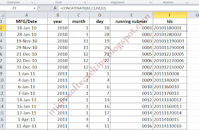
5. type =concatenate(B2,C2,D2,E2). Drag or copy paste the formula all the way (to cover the all the dates)

Note that the ids are not of the same length. 

To avoid you can use IF and LEN as described below.

2a. type =IF(LEN(MONTH(A2))=1,CONCATENATE("0",MONTH(A2)),MONTH(A2)) in column C 

3a. type =IF(LEN(DAY(A2))=1,CONCATENATE("0",DAY(A2)),DAY(A2)) in Column D

The result will be as follows

Here we go nice and clean IDs.

Done.

All comments are welcome.