Preparing Data for Stacked Column Chart in Excel

I recently had a situation where I have part measured repeatedly after rework. The number of times the each parts measured and which  measurement belongs to which rework is only can be identified by "time stamp" (the time of the measurement). Please refer to the sample data. Please note the data is sort by time stamp and part name. 

Now I need to a Stacked Column Chart like below. This is to have visual representation of the effect of rework. My original intention to use Qliksense or Tableau but excel can do the job with an additional table. 

Step 1: First sort the table by part and then by time stamp. 

Step 2: Add a column (column D) with the formula

="Measurement No" & COUNTIF(B$2:B2,B2)

Step 3: Drag the formula all the way.

Step 4: Now you can create the table for the Stacked Column Chart.

The table should be like the image below.

Add formula =SUMIFS($C:$C,$B:$B,J$1,$D:$D,$I2) in cell J2.

Fill the table with the formula.

Use insert → chart → stacked column to create the chart.

Arranging names in alphabetical order and placing them under the alphabet

Lets say we have 50 names and the names to be put under them starting alphabet in alphabetical order.

Below is the sample of names.

Sample of expected results, names under their respective first letter.

OK, lets see how to do this.

In this example names are in worksheet 1.
I am going use another sheet (sheet 2) for the intermediate sorting and worksheet 3 for the final results.

In the intermediate sorting, I will list the names under each alphabets, but not in sorted.

In sheet 2 lets key in Alphabets (A, B, C, ....) in alternate columns as shown below. Make sure to have a empty column before the column with  alphabet A.

In C2 key in =IF(LEFT(Sheet1!$D2,1)=Sheet2!C$1,Sheet1!$D2,"ZZZZZ") H

Lets take a look at the formula and analyse what it does.

The condition for the IF function is LEFT(Sheet1!$D2,1)=Sheet2!C$1. I am just taking the first letter of the name and comparing against the Alphabet, in this case "A".

The result if "TRUE" is the name (in the corresponding row) in Sheet 1. The result if "FALSE" is "ZZZZZ". Why "ZZZZZ"? Let me explain later.

Note:  How to use LEFT command please refer to this post. http://newexceltips.blogspot.sg/2012/06/how-to-use-date-right-and-left-formulas.html

Drag the formula as needed. The result is like shown below.

As you can see the names appear under their respective first alphabet. But there are lots of "ZZZZZ" and the names are not sorted A-Z.

Now I make use of the empty column in-front of every column with names. For example for column C which contains names starting with" A" I use cell B2 to key in the following formula.

=COUNTIF(Sheet2!C$2:C$51,"<="&Sheet2!C2)

This formula will give numbers corresponding to the name in the list. For example if we have name AA, AZ and AD, the corresponding numbers will be 1, 3 and 2. This is exactly what a alphabetical sorting order should be. So "ZZZZZ" will be given max value, in this example 50.

In another sheet you can have Alphabets on one row and use VLOOKUP to pull the names in the sorted order.

The Vlookup command is (in cell B2)

=VLOOKUP(ROW(B2)-ROW(B$1),Sheet2!B:C,2,FALSE)

Notice the error in cell B6 onwards after dragging the formula.
To correct this add a IFERROR formula to VLOOKUP formula.

=IFERROR(VLOOKUP(ROW(B2)-ROW(B$1),Sheet2!B:C,2,FALSE),"")


Now extend the formula to all the alphabets (A-Z) to complete the table.

If any addition of names in the original list will be updated automatically (the formula range should cover the cell).  For example add "Aann". 

Please leave your comments.

How to find duplicates in column without deleting them

It is a common requirement to find duplicates, in most cases the duplicates need to be deleted, but in some cases the duplicates need to be kept.

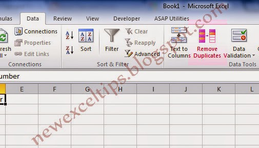
Excel 2010 (even 2007?) got the feature under "DATA" to remove duplicate entries in column(s), called Remove Duplicates. 

 

The issue with this tool it removes the duplicates and do not give more details.

If you want to mark the duplicates or want to VLOOKUP unique values you need use COUNTIF.

Let's see the example below, 

There are many duplicate entries i  column D. If you want to put "Duplicate" in column C, use

=IF(COUNTIF($D$2:$D$45,D2)>1,"DUPLICATE","")

The result will be,

Important to note, if there is two or more values, all considered "DUPLICATE". This will not help if you are looking to use unique values. For example if you try to index the unique values, let's say in column B.

You may want to use,

=IF(C2="DUPLICATE","",MAX(B$1:B1)+1)

The result will be a "1" in B15. In other words there is only one unique value in column D. But we know it is not true. To solve this we need to change the COUNTIF slightly.

Instead of 

=IF(COUNTIF($D$2:$D$45,D2)>1,"DUPLICATE","")

We will use, 

=IF(COUNTIF(D$2:D2,D2)>1,"DUPLICATE","")

and the result is,

Now you can use VLOOKUP to pull the unique values, Vlookup(1,B:D,2,FALSE) and so on.

The Key Point is to leave the first instance of the duplicates as "Unique".



There will be lot of other ways to do the same. 
I will be happy to have any feedback.

How to use COUNTIFS

In an earlier post  I discussed about using CONCATENATE and COUNTIF to sum with two conditions. This can be done using the new COUNTIFS command.

Lets look at the following example:

I need to know the number of times machine 9 was used on  4th Jan 2011.

Use formula,

=COUNTIFS(F:F,DATE(2011,1,4),G:G,9)

You can use up to 127 criteria

DONE.

How to use CONCATENATE and COUNTIF together

Prerequisite 

Know how to use "CONCATENATE" and "COUNTIF" individually. Please refer to Microsoft help for 

Syntax. 

What is concatenation means, please read here, http://en.wikipedia.org/wiki/Concatenation.
Simply put join two or more words.


Simple Example 

Lets consider a simple scenario,

Data given (raw data) : quantity produced by different machines on different days

Data needed : Number of times (frequency) each machine used on each date.

The steps (How to do)

Stap 1: Create a new column to join date and machine using "Concatenate".

  

Note: I am using  "-" to make sure no duplicates.

the formula in column (refer to the image) is  =CONCATENATE(N3,"-",O3).

Make sure the formula is dragged to all the way to the bottom of the table.

Step 2: create the matrix 

Manufacturing date in the column and machines in the raw (it can be done vise-verse also)

Step 3: formula to calculate the total quantity produced by each machines on different days.

Use" COUNTIF" to do the calculation. Lets start in cell B3.


range    Required. Column M (where the concatenate values are)
criteria    Required. CONCATENATE($A3,"-",B$2)

Let's focus on CONCATENATE($A3,"-",B$2). This formula is the same as in column M. The main difference in freezing column and raw values. $A3 is column freeze and  B$2 is raw freeze. The freezing allow us to drag the formula.

Step 4: Drag the formula to fill up the entire table

DONE

Step 5: Check and Balance

Always good to do a check on the accuracy.

In this case SUM(B3:J12) sould be equal to COUNT(P:P)