How to use CONCATENATE to create TAG or Labels

Prerequisite 

Know how to use "CONCATENATE", "MAX", and "IF" individually. Please refer to Microsoft help for 

Syntax. 

What is concatenation means, please read here, http://en.wikipedia.org/wiki/Concatenation.
Simply put join two or more words.

Possible Usage

1. blogging - For those doing blogging regularly for tagging or labeling

2. Tagging for photo (like when you upload to Photobucket etc...)

The steps (How to do)

1. Key in the tags or labels in a column. Please note that the first raw is not used.

2. In cell A2 key in the formula, =IF(B2="A",MAX(A$1:A1)+1,"")

3. Drag or copy paste the formula all the way (to cover the all the tags or labels)

4. Key in "A" in column B in the corresponding raw you need.

5. In column E, key in =max(A:A)

6. In cell F2 type "1"

7. In cell F3 type =IF($E$1<=F2,"",F2+1)

8. Drag or copy paste the formula all the way (to cover the all the tags or labels)

9. In Cell G2 key in formula =IF(F2="","",VLOOKUP(F2,A:C,3,FALSE))

10. Drag or copy paste the formula all the way (to cover the all the tags or labels)

11. In cell H2 key in =CONCATENATE(G2,",",G3,",",G4,",",G5,",",G6,",",G7,",",G8,",",G9,",",G10,",",G11)

12. copy the content to the blogger or any other site

DONE

How to use CONCATENATE and COUNTIF together

Prerequisite 

Know how to use "CONCATENATE" and "COUNTIF" individually. Please refer to Microsoft help for 

Syntax. 

What is concatenation means, please read here, http://en.wikipedia.org/wiki/Concatenation.
Simply put join two or more words.


Simple Example 

Lets consider a simple scenario,

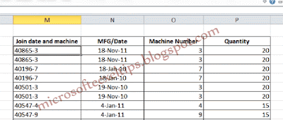
Data given (raw data) : quantity produced by different machines on different days

Data needed : Number of times (frequency) each machine used on each date.

The steps (How to do)

Stap 1: Create a new column to join date and machine using "Concatenate".

  

Note: I am using  "-" to make sure no duplicates.

the formula in column (refer to the image) is  =CONCATENATE(N3,"-",O3).

Make sure the formula is dragged to all the way to the bottom of the table.

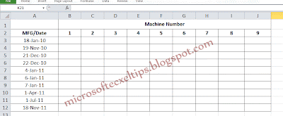
Step 2: create the matrix 

Manufacturing date in the column and machines in the raw (it can be done vise-verse also)

Step 3: formula to calculate the total quantity produced by each machines on different days.

Use" COUNTIF" to do the calculation. Lets start in cell B3.


range    Required. Column M (where the concatenate values are)
criteria    Required. CONCATENATE($A3,"-",B$2)

Let's focus on CONCATENATE($A3,"-",B$2). This formula is the same as in column M. The main difference in freezing column and raw values. $A3 is column freeze and  B$2 is raw freeze. The freezing allow us to drag the formula.

Step 4: Drag the formula to fill up the entire table

DONE

Step 5: Check and Balance

Always good to do a check on the accuracy.

In this case SUM(B3:J12) sould be equal to COUNT(P:P)

How to use CONCATENATE and SUMIF together

Prerequisite 

Know how to use "CONCATENATE" and "SUMIF" individually. Please refer to Microsoft help for 

Syntax. 

What is concatenation means, please read here, http://en.wikipedia.org/wiki/Concatenation.
Simply put join two or more words.


Simple Example 

Lets consider a simple scenario,

Data given (raw data) : quantity produced by different machines on different days

Data needed : mapping (matrix) qty produced by different machines on different days.

The steps (How to do)

Stap 1: Create a new column to join date and machine using "Concatenate".

  

Note I am using  "-" to make sure no duplicates.

the formula in column (refer to the image) is  =CONCATENATE(N3,"-",O3).

Make sure the formula is dragged to all the way to the bottom of the table.

Step 2: create the matrix 

Manufacturing date in the column and machines in the raw (it can be done vise-verse also)

Step 3: formula to calculate the total quantity produced by each machines on different days.

Use sumif to do the calculation. Please note the range column and sum_range column are different. Lets start in cell B3.


range    Required. Column M (where the concatenate values are)
criteria    Required. CONCATENATE($A3,"-",B$2)
sum_range     Required . Column P

Let's focus on CONCATENATE($A3,"-",B$2). This formula is the same as in column M. The main difference in freezing column and raw values. $A3 is column freeze and  B$2 is raw freeze. The freezing allow us to drag the formula.

Step 4: Drag the formula to fill up the entire table

DONE

Step 5: Check and Balance

Always good to do a check on the accuracy.

In this case SUM(B3:J12) sould be equal to SUM(P:P)




This is my first post in this blog let me know your thoughts.