Create year , quarter , month, Week, day, hour

 We often need to do summary reports based on week, month, quarter, year and so on. 

Let's see how to extract these info from time stamp.

For example lets consider 1/1/2021  4:00:00 AM

Hour

=TEXT(A2,"hh")

Day

=TEXT(A2,"dd")

=TEXT(A2,"ddd")

=TEXT(A2,"dddd")

Week

=WEEKNUM(A2)

Month

=TEXT(A2,"mm")

=TEXT(A2,"mmm")

=TEXT(A2,"mmmm")

Quarter

To calculate quarter we will use month info.

=ROUNDUP((MONTH(A2))/3,0)

Some companies use different starting month for quarter need to adjust the month.

Year

=TEXT(A2,"yyyy")

Preparing Data for Stacked Column Chart in Excel

I recently had a situation where I have part measured repeatedly after rework. The number of times the each parts measured and which  measurement belongs to which rework is only can be identified by "time stamp" (the time of the measurement). Please refer to the sample data. Please note the data is sort by time stamp and part name. 

Now I need to a Stacked Column Chart like below. This is to have visual representation of the effect of rework. My original intention to use Qliksense or Tableau but excel can do the job with an additional table. 

Step 1: First sort the table by part and then by time stamp. 

Step 2: Add a column (column D) with the formula

="Measurement No" & COUNTIF(B$2:B2,B2)

Step 3: Drag the formula all the way.

Step 4: Now you can create the table for the Stacked Column Chart.

The table should be like the image below.

Add formula =SUMIFS($C:$C,$B:$B,J$1,$D:$D,$I2) in cell J2.

Fill the table with the formula.

Use insert → chart → stacked column to create the chart.

How to use "INDIRECT" function

Lets say we have production log sheet for technicians to put a "x" in the relevant cell, as shown below. Technicians assigned working on the particular date enters a cross "x" in the corresponding row and corresponding column (his/her name).

Then we need to get all the names in column C. This will be very help full in many ways. 

Use formula in cell C2 and populate as needed. 

=INDIRECT(ADDRESS(2,MATCH("x",D3:K3,0)+COLUMN()))

Lets analyse the formula, 

1. INDIRECT needs the cell reference.

2. To get the reference cell I am using ADDRESS function. Address function requires row number and column number.

3. Row number is 2, as that is the contains name of the technicians.

4. Column number is bit complicated. Use MATCH function to find the column number within the selected range (in this example D3:K3). Use COLUMN function to find the column number where the result to be displayed (column C in this example).  

MATCH("x",D3:K3,0)+COLUMN()

The result will be like image below,

Comments are welcome.

How to use AVERAGEIF and AVERAGEIFS

In the earlier posts we have looked at using SUMIF, SUMIFS, COUTIF AND COUNTIFS. In this post lets see how to use AVERAGEIF and AVERAGEIFS, 

Lets look at the following example:

Let say I need to calculate the average quantity produced for each day.

First make a list of dates (unique).

=AVERAGEIF(E:E,A3,G:G)

Extend the formula as needed.

Let say i need the average by machine (1 to 9) and date then i need to use AVERAGEIFS. 

The results will be,

The formula is 

=AVERAGEIFS($U:$U,$S:$S,$A3,$T:$T,B$2)

Please note the quantity is in column U, dates in column S and machine number in column T.

I have added IFERROR function to get rid of #DIV/0! error

=IFERROR(AVERAGEIFS($U:$U,$S:$S,$A3,$T:$T,B$2),"")

Please leave your comments, thanks.

How to use formulas with Chart titles

This is a very simple trick but seems many not aware of it. Let say we need a chart for daily production out put and the data is updated every day.

Lets add (insert) a bar chart.

Select the data

Insert chart

The chart looks like,

Now need to add some titles for horizontal and vertical axis. 

Select "DESIGN" from menu → select "Add Chart Element" → select "Axis Titles" → select "Primary Horizontal"

Do the above for "Primary Vertical" also.

The chart will look like,

Now change the "Axis Title". 

Click on the Horizontal "Axis Title" and in the "Formula Bar" type =Sheet1!$B$5. 

For vertical axis title type =Sheet1!$C$5.

Now the chart looks like,

Now, Chart title need to be changed to "Output report for 25 January 2014" and if the data changed to another date the chart title to be changed accordingly.  This is where we need a bit more complicated formula. 

In a cell (E1) key in the following formula

=CONCATENATE("Output Report for ",(CONCATENATE(DAY($C$3)," ",TEXT($C$3,"mmmm")," ",YEAR($C$3))))

(CONCATENATE(DAY($C$3)," ",TEXT($C$3,"mmmm")," ",YEAR($C$3)))) = 25 January 2014

Please pay attention to the month "TEXT($C$3,"mmmm")" formula. 

Then click on the chat title and key in =Sheet1!$E$1 in the formula bar.

Now the chart will look like,

Now if the data changed to 1 March 2014, the chart will be changed automatically,

Please leave your comments, thanks.

Arranging names in alphabetical order and placing them under the alphabet

Lets say we have 50 names and the names to be put under them starting alphabet in alphabetical order.

Below is the sample of names.

Sample of expected results, names under their respective first letter.

OK, lets see how to do this.

In this example names are in worksheet 1.
I am going use another sheet (sheet 2) for the intermediate sorting and worksheet 3 for the final results.

In the intermediate sorting, I will list the names under each alphabets, but not in sorted.

In sheet 2 lets key in Alphabets (A, B, C, ....) in alternate columns as shown below. Make sure to have a empty column before the column with  alphabet A.

In C2 key in =IF(LEFT(Sheet1!$D2,1)=Sheet2!C$1,Sheet1!$D2,"ZZZZZ") H

Lets take a look at the formula and analyse what it does.

The condition for the IF function is LEFT(Sheet1!$D2,1)=Sheet2!C$1. I am just taking the first letter of the name and comparing against the Alphabet, in this case "A".

The result if "TRUE" is the name (in the corresponding row) in Sheet 1. The result if "FALSE" is "ZZZZZ". Why "ZZZZZ"? Let me explain later.

Note:  How to use LEFT command please refer to this post. http://newexceltips.blogspot.sg/2012/06/how-to-use-date-right-and-left-formulas.html

Drag the formula as needed. The result is like shown below.

As you can see the names appear under their respective first alphabet. But there are lots of "ZZZZZ" and the names are not sorted A-Z.

Now I make use of the empty column in-front of every column with names. For example for column C which contains names starting with" A" I use cell B2 to key in the following formula.

=COUNTIF(Sheet2!C$2:C$51,"<="&Sheet2!C2)

This formula will give numbers corresponding to the name in the list. For example if we have name AA, AZ and AD, the corresponding numbers will be 1, 3 and 2. This is exactly what a alphabetical sorting order should be. So "ZZZZZ" will be given max value, in this example 50.

In another sheet you can have Alphabets on one row and use VLOOKUP to pull the names in the sorted order.

The Vlookup command is (in cell B2)

=VLOOKUP(ROW(B2)-ROW(B$1),Sheet2!B:C,2,FALSE)

Notice the error in cell B6 onwards after dragging the formula.
To correct this add a IFERROR formula to VLOOKUP formula.

=IFERROR(VLOOKUP(ROW(B2)-ROW(B$1),Sheet2!B:C,2,FALSE),"")


Now extend the formula to all the alphabets (A-Z) to complete the table.

If any addition of names in the original list will be updated automatically (the formula range should cover the cell).  For example add "Aann". 

Please leave your comments.

How to use INDEX function - part one

We have seen how to use VLOOKUP in the earlier posts,

http://newexceltips.blogspot.sg/2012/07/how-to-use-column-and-columns-functions.html and 

http://newexceltips.blogspot.sg/2012/05/how-to-use-concatenate-to-create-tag-or.html.

In the same way we can use HLOOkUP (vertical and horizontal).


But if we need to use vertical and horizontal look up at the same time, we need to use INDEX. 
Lets say we have table like below,

and say we need to make a table like below,

In the cell J3, type =INDEX( and choose 

As you can see we need an array (table), row number and column number. To find corresponding row number and column number we need to use Formula "MATCH".

for example 

Row number MATCH(H3,A3:A11,0)
Column number MATCH(I3,B2:E2,0)

Lets look how the formula looks like,

Note the row number and column number needed are of the array (table) not of the worksheet.


So here is the formula,
=INDEX(B3:E11,MATCH(H3,A3:A11,0),MATCH(I3,B2:E2,0))

As usual we need to lock the cells.
=INDEX($B$3:$E$11,MATCH($H3,$A$3:$A$11,0),MATCH($I3,$B$2:$E$2,0))

Then drag the the formula to the cells as needed.



We can also use as array formula. 
=INDEX($B$3:$E$11,MATCH(H3:H5,$A$3:$A$11,0),MATCH(I3:J5,$B$2:$E$2,0))
Remember to use Shift+Ctrl+Enter

If we are expecting wrong Machine or Data (accidental or otherwise) then we can add a 

IFERROR (Excel 2007 onwards).
=IFERROR(INDEX($B$3:$E$11,MATCH($H6,$A$3:$A$11,0),MATCH($I6,$B$2:$E$2,0)),"NO VALUE")

or ISERROR (Old versions of Excel)
=IF(ISERROR(INDEX($B$3:$E$11,MATCH($H6,$A$3:$A$11,0),MATCH($I6,$B$2:$E$2,0)))=TRUE,"NO VALUE",INDEX($B$3:$E$11,MATCH($H6,$A$3:$A$11,0),MATCH($I6,$B$2:$E$2,0)))

  

That's it. Your comments are always welcome.

How to split a cell diagonally

Let say we need to split the cells diagonally. Mainly when we want make a nice looking table.

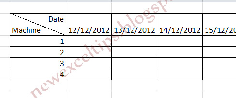
Let say we need a table showing machine numbers and outputs per day.

As you can see event though the data can be represented properly, the presentation part is not very good as there will be empty cells (colored in yellow).

A nicer table should have "Date" and "Machine" in the same cell. Just like the one below,

Let see how to do this.

1. Right click on the cell where we want to put "Date" and "Machine" and click on Format cells.

Select "Border" and click on the diagonal border.

Click "OK"

Set the cell's Horizontal Alignment to "left" and vertical alignment to "center".

Type in "Date" then Hit "Alt+Enter". The type in "Machine".

Use the space bar to push the "Date" to right to get what we want.




If you want to have two colors for the split area you can try the "Fill effects". Choose "two colors" and "Diagonal Down". This is the best I can think of.

Please note if you want to use the value (date machine), this is not the method. 

As always love to have your comments.